
Tidy Data
Original Author: Nic Weber
Editing & Updates: Bree Norlander
The idea of “tidy data” underlies principles in data management, and database administration that have been around for decades. In 2014, Hadley Wickham started to formalize some of these rules in what he called “Principles for Tidy Data.” PDF
These principles are focused mainly on how to follow some simple conventions for structuring data in a matrices (or tables) to use in the statistical programming language R.
In this module, I am going to give an overview of tidy data principles as they relate to data curation, but also try to extend “tidy data” to some of the underlying principles in organizing, managing, and preparing all kinds of structured data for meaningful use. This module will be relevant again in module 8 when we discuss tidy metadata.
Tidy Data Principles
The foundation of Wickham’s “Tidy Data” relies upon a definition of a single table which contains (Wickham, p. 3, 2014):
- A collection of values, and every value belongs to a corresponding variable (column) and observation (row).
- A variable (column), contains all values that measure the same attribute (such as height, temperature, duration) across all units (observations/rows).
- An observation (row), contains all values measured on the same unit (such as a person, a date, a state) across all attributes (variables/columns).
It also allows for the creation of relationships with multiple tables with this principle:
- Each type of observational unit forms a table.
We will be focused on tidying a single table for most of this module, but you can see an example of multiple tables in the R for Data Science section on relational data in the NYC Flights dataset.
Put simply, for any given table we associate one observation with one or more variables. Each variable in a tidy dataset has a standard unit of measurement for its values.
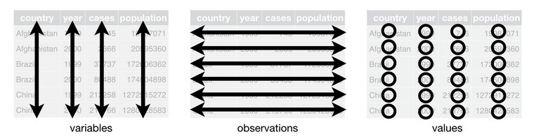
This image depicts the structure of a tidy dataset.
The following tidy data table includes characters appearing in a Lewis Caroll novel. The characters are observations, and the variables that we associate with each observation are Age and Height. Each variable has a standard unit of measurement.
| Name | Age | Height |
|---|---|---|
| Bruno | 22 years | 61 inches |
| Sylvie | 23 years | 62 inches |
Tidy Data Curation
The principles described above may seem simplistic and highly intuitive. But, often these principles aren’t followed when creating or publishing a dataset. This may be for a variety of reasons, but most obvious is that data creators are often working for convenience in data entry rather than thinking about future data analysis.
Think back to our module 2 example of an ecology graduate student sitting in a field observing frogs. After a long day of fieldwork she might not care too much about how she makes her data conform with principles of tidy data, she just wants to record her observations. Or, she may be simply following the conventions of a structure that has already been set up by a member of her lab. Later, when she returns to the data to perform some analysis for a publication she may need to clean the data in order to ease computation. But, often she’ll simply archive her raw data and not worry about what she did to transform the data in order to make it useful for analysis. These data management practices are highly inefficient, and represent an excellent point for curators to intervene.
For data curators, the principles of tidy data can be applied at different points in time.
-
Upstream tidying: In working “upstream” a data curator is collaboratively developing standards to govern data collection and management. In this proactive work a data curator can advocate for these principles at the point in which data is initially made digital.
-
Downstream tidying: More commonly, a data curator will receive some untidy data after it has been collected and analyzed. Working downstream requires tidying, such as restructuring and standardizing data, so that it adheres to the principles described above.
In working downstream, there are some additional data transformations that are helfpul for adhering to tidy data principles. These include using pivots to widen or make data longer, and separating or gathering data into a single variable.
Pivoting data
A pivot table is commonly used to summarize data in some statistical way so as to reduce or summarize information that may be included in the original table. In describing the “pivot” as it applies to a tidy dataset, there are two common problems that this technique can help solve.
First, a variable is often inefficently “spread” across multiple columns. For example, we may have the observation of a country and a variable like GDP that is represented annually. Our dataset could look like this:
| Country | 2016 | 2017 |
|---|---|---|
| USA | 18.71 | 19.49 |
| UK | 2.69 | 2.66 |
The problem with this structure is that the GDP variables are currently represented as annual values. That is, we have variables that are spread out across multiple columns when they could be easily and more effectively included as values for multiple observations.
To tidy this kind of dataset we would transform the data by using a long pivot. We will restructure the data table so that it is longer - containing more observations. To do this we will:
- Create a
Yearcolumn that can represent the year in which the GDP is being observed for a country. - Create a second column that can represent the GDP value.
- We will then separate the observations based on the year in which they occur.
Our new tidy dataset then looks like this:
| Country | Year | GDP |
|---|---|---|
| USA | 2016 | 18.71 |
| UK | 2016 | 2.69 |
| USA | 2017 | 19.49 |
| UK | 2017 | 2.66 |
Our dataset now contains four observations: USA 2016, USA 2017, UK 2016, and UK 2017. What we’ve done is remove any external information needed to interpret what the data represent. This could, for example, help with secondary analysis when we want to directly plot GDP over time.
The second type of data structuring problem that curators are likely to encounter is when one observation is scattered across multiple rows. This is the opposite of the problem that we encountered with variables spread across multiple columns. In short, the problem with having multiple observations scattered across rows is that we’re duplicating information by confusing a variable for a value.
| Country | Year | Measure | Number |
|---|---|---|---|
| USA | 2016 | GDP | 18.71 trillion USD |
| USA | 2016 | Population | 323.1 million people |
| UK | 2016 | GDP | 2.69 trillion USD |
| UK | 2016 | Population | 65.38 million people |
It should be obvious that we are not abiding by tidy data principles in at least one respect. The variable (column), Number, does not contain a single unit of measurement. Instead it contains two different measurements, “USD” and “count of people”. Additionally, the variable (column), Measure, contains multiple values, “GDP” and “Population.” To tidy this kind of dataset we will use a wide pivot. We will restructure the data so that each column corresponds with one variable, and each variable contains a value of a single unit of measurement.
| Country | Year | GDP | Population |
|---|---|---|---|
| USA | 2016 | 18.71 | 323.1 |
| UK | 2016 | 2.69 | 65.38 |
Our dataset now contains only two observations - the GDP and Population for the UK and USA in 2016. But, note that we also solved a separate problem that plagues the scattering of observations. In the first dataset we had to declare, in the Number column, the unit of measurement. GDP is measure in the trillions of USD and Population is measured in the millions of count of people. Through our wide pivot transformation we now have a standard measurement unit for each variable, and no longer have to include measurement information in our values. (One reason this is important is that the value can now have a data type that is useful for performing mathematics. Originally, the value was a combination of a number (e.g. type = numeric) and words (e.g. type = string). Most data analysis tools will coerce the entire value into a string/character and the user will not be able to perform calculations.) In this example we have not included the metadata about the variable. Ideally, we would either conform to a metadata schema that specifies units, or include a data dictionary indicating the standard unit of measurement, or we state it explicitly in the column heading (such as GDP_USD_trillions). How you indicate the units of measurement will vary depending on your domain and the standard practices in your setting.
In sum, the pivot works to either:
- Transform variables so that they correspond with just one observation. We do this by adding new observations. This makes a tidy dataset longer.
- Transform values that are acting as variables. We do this by creating new variables and replacing the incorrect observation. This makes a tidy dataset wider.
Separating and Gathering
Two other types of transformations are often necessary to create a tidy dataset: Separating values that may be incorrectly combined, and Gathering redundant values into a single variable. Both of these transformations are highly context dependent.
Separating
Separating variables is a transformation necessary when two distinct values are used as a summary. This is a common shorthand method of data entry.
| Country | Year | GDP per capita |
|---|---|---|
| USA | 2016 | 18710/0.3231 |
| UK | 2016 | 2690/0.06538 |
In this table we have a variable GDP per capita that represents the amount of GDP divided by the population of each country (the numbers have changed from the previous examples to standardize the units of measurement). This may be intuitive to an undergraduate economics student, but it violates our tidy data principle of having one value per variable. Also notice that the GDP per capita variable does not use a standard unit of measurement and includes a character (string) /.
To separate these values we would simply create a new column for each of the variables. You may recognize this as a form of ‘wide pivot’.
| Country | Year | GDP | Population | GDP per Capita |
|---|---|---|---|---|
| USA | 2016 | 18710 | 0.3231 | 57908 |
| UK | 2016 | 2690 | 0.06538 | 41144 |
By separating the values into their own columns we know have a tidy dataset that includes four variables for each observation. Again, the explanation of units of measurement and the calculation used to creat the “GDP per capita” column should be included in the metadata.
Gathering
Gathering variables is the exact opposite of separating - instead of having multiple values in a single variable, a data collector may have gone overboard in recording their observations and unintentionally created a dataset that is too granular (that is, has too much specificity). Generally, granular data is good - but it can also create unnecessary work for performing analysis or interpreting data when taken too far.
| Species | Hour | Minute | Second | Location |
|---|---|---|---|---|
| Aparasphenodon brunoi | 09 | 58 | 10 | Brazil |
| Aparasphenodon brunoi | 11 | 22 | 17 | Honduras |
In this dataset we have a very granular representation of time. If, as data curators, we wanted to represent time using a common standard like ISO 8601 (and we would, because we’re advocates of standardization) then we need to gather these three distinct variables into one single variable. This gathering transformation will represent, in a standard way, when the species was observed (Yes, this frog’s common name is “Bruno’s casque-headed frog” - I have no idea whether or not this is related to the Lewis Caroll novel, but I like continuity.)
| Species | Time of Observation | Location |
|---|---|---|
| Aparasphenodon brunoi | 09:58:10 | Brazil |
| Aparasphenodon brunoi | 11:22:17 | Honduras |
Our dataset now has just two variables - the time when a species was observed, and the location. We’ve appealed to standard (IS0 8601) to represent time, and expect that anyone using this dataset will know the temporal convention HH:MM:SS. And, we assume that the timezone is standardized and stated in the metadata (otherwise we would need a column for timezone).
As I said in opening this section - the assumptions we make in tidying data are highly context dependent. If we were working in a field where granular data like seconds was not typical, this kind of representation might not be necessary. But, if we want to preserve all of the information that our dataset contains then appealing to broad standards is a best practice.
Tidy Data in Practice
For the purposes of this class, using tidy data principles in a specific programming language is not necessary. Simply understanding common transformations and principles are all that we need to start curating tidy data.
But, it is worth knowing that the tidy data principles have been implemented in a number of executable libraries using R. This includes the suite of libraries known as the tidyverse. A nice overview of what the tidyverse libraries make possible working with data in R is summarized in this blogpost by Joseph Rickert. (Note from Bree: I love R and use it everyday!)
There are also a number of beginner tutorials and cheat-sheets available to get started. If you come from a database background, I particularly like this tutorial on tidy data applied to the relational model by my colleague Iain Carmichael.
Extending Tidy Data Beyond the Traditional Observation
Many examples of tidy data, such as the ones above, depend upon discrete observations that are often rooted in statistical evidence, or a scientific domain. Qualitative and humanities data often contain unique points of reference (e.g. notions of place rather than mapped coordinates), interpreted factual information (e.g. observations to a humanist mean something very different than to an ecologist), and a need for granularity that may seem non-obvious to the tidy data curator.
In the following section I will try to offer some extensions to the concept of tidy data that draws upon the work of Matthew Lincoln for tidy digital humanities data (see an example of one of Matthew’s workshops here). In particular, we will look at ways to transform two types of data: Dates and Categories. Each of these types of data often have multiple ways of being represented. But, this shouldn’t preclude us from bringing some coherence to untidy data.
For these explanations I’ll use Matthew’s data because it represents a wonderful example of how to restructure interpreted factual information that was gathered from a museum catalog. The following reference dataset will be used throughout the next two sections. Take a quick moment to read and think about the data that we will transform.
| acq_no | museum | artist | date | medium | tags |
|---|---|---|---|---|---|
| 1999.32 | Rijksmuseum | Studio of Rembrandt, Govaert Flink | after 1636 | oil on canvas | religious, portrait |
| 1908.54 | Victoria & Albert | Jan Vermeer | 1650 circa | oil paint on panel | domestic scene and women |
| 1955.32 | British Museum | Possibly Vermeer, Jan | 1655 circa | oil on canvas | woman at window, portrait |
| 1955.33 | Rijksmuseum | Hals, Frans | 16220 | oil on canvas, relined | portraiture |
Dates
In the previous section I described the adherence to a standard, ISO 8601, for structuring time based on the observation of a species. We can imagine a number of use cases where this rigid standard would not be useful for structuring a date or time. In historical data, for example, we may not need the specificity of an ISO standard, and instead we may need to represent something like a time period, a date range, or an estimate of time. In the museum catalog dataset we see three different ways to represent a date: After a date, circa a year, and as a data error in the catalog (16220).
It is helpful to think of these different date representations as “duration” (events with date ranges) and “fixed points” in time.
Following the tidy data principles, if we want to represent a specific point in time we often need to come up with a consistent unit of measurement. For example, we may have a simple variable like date with the following different representations:
| Date |
|---|
| 1900s |
| 2012 |
| 9th century |
Here we have three different representations of a point in time. If we want to tidy this data we will have to decide what is the most meaningful representation of this data as a whole. If we choose century, as I would, then we will have to sacrifice a bit of precision for our second observation. The benefit is that we will have consistency in representing the data in aggregate.
| Date_century |
|---|
| 20 |
| 21 |
| 9 |
But now, let’s assume that this tradeoff in precision isn’t as clear. If, for example, our dataset contains a date range (duration) mixed with point in time values, then we need to do some extra work to represent this information clearly in a tidy dataset.
| Date |
|---|
| Mid 1200s |
| 9th century |
| 19-20th c. |
| 1980's |
This data contains a number of different estimates about when a piece of art may have been produced. The uncertainty along with the factual estimate is what we want to try to preserve in tidying the data. An approach could be to transform each date estimate into a range.
| date_early | date_late |
| 1230 | 1270 |
| 800 | 899 |
| 1800 |
1999 |
| 1980 | 1989 |
Our data transformation preserves the range estimates, but attempts to give a more consistent representation of the original data. Since we don’t know, for example, when in the mid-1200’s a piece was produced, we infer a range and then create two columns - earliest possible date, and latest possible date - to convey that information to a potential user.
Another obstacle we may come across in representing dates in our data is missing or non-existent data.
| Date |
|---|
| 2000-12-31 |
| 2000-01-01 |
| 1999-12-31 |
| 1999-01 |
We may be tempted to look at these four observations and think it is a simple data entry error - the last observation is clearly supposed to follow the sequence of representing the last day in a year, and the first day in a year. But, without complete knowledge we would have to decide whether or not we should infer this pattern or whether we should transform all of the data to be a duration (range of dates).
There is not a single right answer. A curator would simply have to decide how and in what ways the data might be made more meaningful for reuse. The wrong approach though would be to leave the ambiguity in the dataset. Instead, what we might do is correct what we assume to be a data entry error and create documentation which conveys that inference to a potential reuser.
There are many ways to do this with metadata, but a helpful approach might be just to add a new column with notes.
| Date |
Notes |
|---|---|
| 2000-12-31 | |
| 2000-01-01 | |
| 1999-12-31 | |
| 1999- 01-01 | Date is inferred. The original entry read "1999-01" |
Documentation is helpful for all data curation tasks, but is essential in tidying data that may have a number of ambiguities.
Let’s return to our original dataset and clean up the dates following the above instructions for tidying ambiguous date information.
| acq_no | original_date | date_early | date_late |
|---|---|---|---|
| 1999.32 | after 1636 | 1636 | 1669 |
| 1908.54 | 1650 circa | 1645 | 1655 |
| 1955.32 | 1655 circa | 1650 | 1660 |
| 1955.33 | 16220 | 1622 | 1622 |
We have added two new variables which represent a duration (range of time) - the earliest estimate and the latest estimate of when a work of art was created. (You may be wondering why 1669 is the latest date for the first entry. Rembrandt died in 1669. His work definitely had staying power, but I think it’s safe to say he wasn’t producing new paintings after that).
Note that we also retained the original dates in our dataset. This is another approach to communicating ambiguity - we can simply retain the untidy data, but provide a clean version for analysis. I don’t particularly like this approach, but if we assume that the user of this tidy data has the ability to easily exclude a variable from their analysis then this is a perfectly acceptable practice. (Note from Bree: In my work I tend to prefer the approach of keeping the original data and creating a new column/s with the corrected data. Again this is an example of how practice might differ depending on context or domain.)
Categories
LIS research in knowledge organization (KO) has many useful principles for approaching data and metadata tidying, including the idea of “authority control” which we will talk about in depth in coming weeks. In short though, authority control is the process of appealing to a standard way of representing a spelling, categorization, or classification in data.
In approaching interpretive data that may contain many ambiguities, we can draw upon the idea of authority control to logically decide how best to represent categorical information to our users.
A helpful heuristic to keep in mind when curating data with categories is that it is much easier to combine categories later than it is to separate them initially. We can do this by taking some time to evaluate and analyze a dataset first, and then adding new categories later.
Let’s return to our original dataset to understand what authority control looks like in tidy data practice.
| acq_no | medium |
|---|---|
| 1999.32 | oil on canvas |
| 1908.54 | oil paint on panel |
| 1955.32 | oil on canvas |
| 1955.33 | oil on canvas, relined |
In the variable medium there are actually three values:
- The medium that was used to produce the painting.
- The material (or support) that the medium was applied to.
- A conservation technique.
This ambiguity likely stems from the fact that art historians often use an informal vocabulary for describing a variable like medium.
Think of the placard on any museum that you have visited – Often the “medium” information on that placard will contain a plain language description. This information is stored in a museum database and used to both identify a work owned by the museum, but also produce things like exhibit catalogues and placards. Here is an example of placard using information represented in our dataset:

But, we don’t want to create a dataset that retains ambiguous short-hand categories simply because this is convenient to an exhibit curator. What we want is to tidy the data such that it can be broadly useful, and accurately describe a particular piece of art.
This example should trigger a memory from our earlier review of tidy data principles - when we see the conflation of two or more values in a single variable we need to apply a “separate” transformation. To do this we will create three new variables to perform a “wide pivot”.
| acq_no | medium | support | cons_note |
|---|---|---|---|
| 1999.32 | oil | canvas | |
| 1908.54 | oil | panel | |
| 1955.32 | oil | canvas | |
| 1955.33 | oil | canvas | relined |
In this wide pivot, we retained the original medium variable, but we have also separated the support and conservation notes into new variables. (Note: I will have much more to say about this example and how we can use an “authority control” in future modules.)
Our original dataset also contained another variable Name with multiple values and ambiguities. In general, names are the cause of great confusion in information science. In part because names are often hard to disambiguate across time, but also because “identity” is difficult in the context of cultural heritage data. Art history is no exception.
In our original dataset, we have a mix of name disambugity and identity problems.
| acq_no | artist |
|---|---|
| 1999.32 | Studio of Rembrandt, Govaert Flink |
| 1908.54 | Jan Vermeer |
| 1955.32 | Possibly Vermeer, Jan |
| 1955.33 | Hals, Frans |
Let’s unpack some of these ambiguities:
- The first observation “Studio of Rembrandt, Govaert Flink” contains two names -
RembrandtandGovaert Flink. It also has a qualification, that the work was produced inthe studio ofRembrandt. - The third observation contains a qualifier
Possiblyto note uncertainty in the painting’s provenance. - All four of the observations have a different way of arranging given names and surnames.
To tidy names there are a number of clear transformations we could apply. We could simply create a first_name and last_name variable and seperate these values.
But this is not all of the information that our Name variable contains. It also contains qualifiers. And, it is much more difficult to effectively retain qualifications in structured data. In part because they don’t neatly fall into the triple model that we expect our plain language to take when being structured as a table.
Take for example our third observation. The subject “Vermeer” has an object (the painting) “View of Delft” being connected by a predicate “painted”. In plain language we could easily represent this triple as “Vermeer painted View_of_Delft”.
But, our first observation is much more complex and not well suited for the triple form. The plain language statement would look somoething like “The studio of Rembrandt sponsored Govaert Flink in painting ‘Isaac blessing Jacob’” (The painting in question is here.)
To represent these ambiguities in our tidy data, we need to create some way to qualify and attribute the different works to different people. Warning in advance, this will be a VERY wide pivot.
| acq_no | artist_1 1stname | artist_1 2ndname |
artist_1 qual |
artist_2 1stname |
artist_2 2ndname |
artist_2 qual |
|---|---|---|---|---|---|---|
| 1999.32 | Rembrandt | studio | Govaert | Flinck | possibly | |
| 1908.54 | Jan | Vermeer | ||||
| 1955.32 | Jan | Vermeer | possibly | |||
| 1955.33 | Hals | Frans |
Across all observations we separated first and second names. In the case of Vermeer, this is an important distinction as there are multiple Vermeers that produced works of art likely to be found in a museum catalogue.
In the third observation, we also added a qualifier “possibly” to communicate that the origin of the work is assumed, but not verified to be Vermeer. We also used this qualification variable for Rembrandt, who had a studio that most definitely produced a work of art, but the person who may have actually put oil to canvas is ambiguous.
We also created a representation of the artist that is numbered - so that we could represent the first artist and the second artist associated with a painting.
Each of these approaches to disambiguation is based on a “separating” transformation through a wide pivot. We tidy the dataset by creating qualifiers, and add variables to represent multiple artists.
This solution is far from perfect, and we can imagine this going quickly overboard without some control in place for how we will name individuals and how we will assign credit for their work (imagine creating the entry for the NAMES Project AIDS Memorial Quilt. But, this example also makes clear that the structural decisions are ours to make as data curators. We can solve each transformation problem in multiple ways. The key to tidy data is having a command of the different strategies for transforming data, and knowing when and why to apply each transformation.
In future chapters we will further explore the idea of appealing to an “authority control” when making these types of decisions around tidying data and metadata.
Summary
In this chapter we’ve gone full tilt on the boring aspects of data structuring. In doing so, we tried to adhere to a set of principles for tidying data:
- Observations are rows that have variables containing values.
- Variables are columns. Each variable contains only one value, and each value follows a standard unit of measurement.
We focused on three types of transformations for tidying data:
- Pivots - which are either wide or long.
- Separating - which creates new variables
- Gathering - which collapses variables
I also introduced the idea of using “authority control” for normalizing or making regular data that does not neatly conform to the conventions spelled out by “Tidy Data Principles”.
Lecture
Readings
Required
- Rowson and Munoz (2016) Against Cleaning: http://curatingmenus.org/articles/against-cleaning/
- Wickham, H. (2014), “Tidy Data,” Journal of Statistical Software, 59, 1–23 https://www.jstatsoft.org/article/view/v059i10/v59i10.pdf (Optional - same article with more code and examples https://r4ds.had.co.nz/tidy-data.html)
Optional
Extending tidy data principles:
- Tierney, N. J., & Cook, D. H. (2018). Expanding tidy data principles to facilitate missing data exploration, visualization and assessment of imputations. arXiv preprint arXiv:1809.02264. (There are a number of very helpful R examples in that paper)
- Leek (2016) Non-tidy data https://simplystatistics.org/2016/02/17/non-tidy-data/
Reading about data structures in spreadsheets:
- Broman, K. W., & Woo, K. H. (2018). Data organization in spreadsheets. The American Statistician, 72(1), 2-10. https://www.tandfonline.com/doi/full/10.1080/00031305.2017.1375989
Teaching or learning through spreadsheets:
- Tort, F. (2010). Teaching spreadsheets: Curriculum design principles. arXiv preprint arXiv:1009.2787.
Spreadsheet practices in the wild:
- Mack, K., Lee, J., Chang, K., Karahalios, K., & Parameswaran, A. (2018, April). Characterizing scalability issues in spreadsheet software using online forums. In Extended Abstracts of the 2018 CHI Conference on Human Factors in Computing Systems (pp. 1-9). Online
Formatting data tables in spreadsheets:
Exercise
Last week you had the opportunity to think about how to transform the traditional layout of a recipe into the form of data. This week, we present to you chocolate chip cookie recipes in “parametric” form from ChefSteps. It appears that the plan was to take a bunch of different recipes and average them. (Creative - Bree would totally try this!) Here is the data behind this infographic in a very messy spreadsheet. Credit to Jenny Bryan for this example of messy data.
This dataset definitely does not meet the definition of “tidy”. There are a number of ways we could restructure this data so that it follows some best practices in efficient and effective reuse. Your assignment is as follows:
- Post to the Canvas discussion board, your thoughts on what should make up the:
- observations (rows)
- variables (columns)
- Test out your choices by creating a sample dataset with at least 3 rows and 3 columns and the associated values. Post your mockup (an Excel spreadsheet, a screenshot, a photo - whatever works).
- Discuss what was easy and difficult about structuring this data.