
Data Integration
Original Author: Nic Weber
Editing & Updates: Bree Norlander
The next four weeks of our class will focus on “grand challenges” in data curation. A grand challenge in this context is a problem that requires sustained research and development activities through collective action. Data integration, packaging, discovery, and meaningful descriptive documentation (metadata) are longstanding grand challenges that are approached through a community of practitioners and researchers in curation. This module focuses on data integration as it operates at the logical level of tables and data that feed into user interfaces.
Integration as a Grand Challenge
In the popular imagination, much of curation work is positioned as the activities necessary to prepare data for meaningful analysis and reuse. For example, when data scientists describe curation work they often say something to the effect of “95% of data science is about wrangling / cleaning.”
If there are only two things I am trying to actively argue against in this class it is this:
- Curation is not just cleaning or wrangling data. It includes the attendant practices of making data contextually meaningful. This includes a good deal of cleaning or wrangling, but is much broader in scope than simply preparing data for analysis.
- Metadata is not just “data about data”. It is a complex and important knowledge organization activity that impacts nearly every aspect of data use. Every time someone says “metadata is just data about data” a tautology angel gets its wings.
In future weeks we will discuss practical ways to approach metadata and documentation that are in line with curation as an activity that goes beyond simply preparing data for analysis. This week, however, we are focused on conceptualizing and approaching the topic of data integration. The combining of datasets is a grand challenge for curation in part because of our expectations for how seemingly obvious this activity should be. Take a moment to consider this at a high level of abstraction: One of the spillover effects of increased openness in government, scientific, and private sector data practices is the availability of more and more structured data. The ability to combine and meaningfully incorporate different information, based on these structures, should be possible. For example:
- All municipalities have a fire department.
- All municipal fire departments have a jurisdictional mandate to proactively investigate fire code compliance.
- It follows, logically, that we should be able to use openly published structured data to look across jurisdictions and understand fire code compliance.
But, in practice this proves to be incredibly difficult. Each jurisdiction has a slightly different fire code, and each municipal fire department records their investigation of compliance in appreciably different ways. So when we approach a question like “fire code compliance” we have to not just clean data in order for it be combined, but think conceptually about the structural differences in datasets and how they might be integrated with one another.
Enumerating data integration challenges
So, if structured data integration is intuitive conceptually, but in practice the ability to combine one or more data sources is incredibly difficult, then we should be able to generalize some of the problems that are encountered in this activity. Difficulties in data integration break down into, at least, the following:
- Content Semantics: Different sectors, jurisdictions, or even domains of inquiry may refer to the same concept differently. In data tidying we discussed ways that data values and structures can be made consistent, but we didn’t discuss the ways in which different tables might be combined when they represent the same concept differently.
- Data Structures or Encodings: Even if the same concepts are present in a dataset, the data may be practically arranged or encoded in different ways. This may be as simple as variables being listed in a different order, but it may also mean that one dataset is published in
CSVanother inJSONand yet another in anSQLtable export. - Data Granularity: The same concept may be present in a dataset, but it may have finer or coarser levels of granularity (e.g. One dataset may have monthly aggregates and another contains daily aggregates).
The curation tradeoff that we’ve discussed throughout both DC 1 and DC 2 in terms of “expressivity and tractability” is again rearing its head. In deciding how any one difficulty should be overcome we have to balance a need for retaining conceptual representations that are accurate and meaningful. In data integration, we have to be careful not go overboard in retaining an accurate representation of the same concept such that it fails to be meaningfully combined with another dataset.
Data Integration, as you might have inferred, is always a downstream curation activity. But, understanding challenges in data integration can also help with decisions that happen upstream in providing recommendations for how data can be initially recorded and documented such that it will be amenable to future integration. (A small plug here for our introductory module - when I described a curator’s need to “infrastructurally imagine” how data will be used and reused within a broader information system, upstream curation activities that forecast data integration challenges are very much what I meant.)
Integration Precursors
To overcome difficulties in combining different data tables we can engage with curation activities that I think of as “integration precursors” - ways to conceptualize and investigate differences in two datasets before we begin restructuring, normalizing, or cleaning. These integration precursors are related to 1. Modeling; 2. Observational depth; and, 3. Variable Homogeneity.
Modeling Table Content
The first activity in data integration is to informally or formally model the structure of a data table. In DC 1 we created data dictionaries which were focused on providing users of data a quick and precise overview of their contents. Data dictionaries are also a method for informally modeling the content of a dataset so that we, as curators, can make informed decisions about restructuring and cleaning.
Here is an example of two data dictionaries for the same conceptual information: 311 service requests to the city of Chicago, IL and Austin, TX (not especially the section called “Columns in this Dataset”). Intuitively, we would expect that data from these two cities are similar enough in content that they can be meaningfully combined.
If we look at the purpose of 311 we should be able to imagine at least a few of the columns, before we even dive into an existing dataset. We can probably safely assume there will be:
- A date
- A report of some service outage or complaint
- A location of the report or complaint, and
- The responsible city service that should respond.
The reality is much messier.
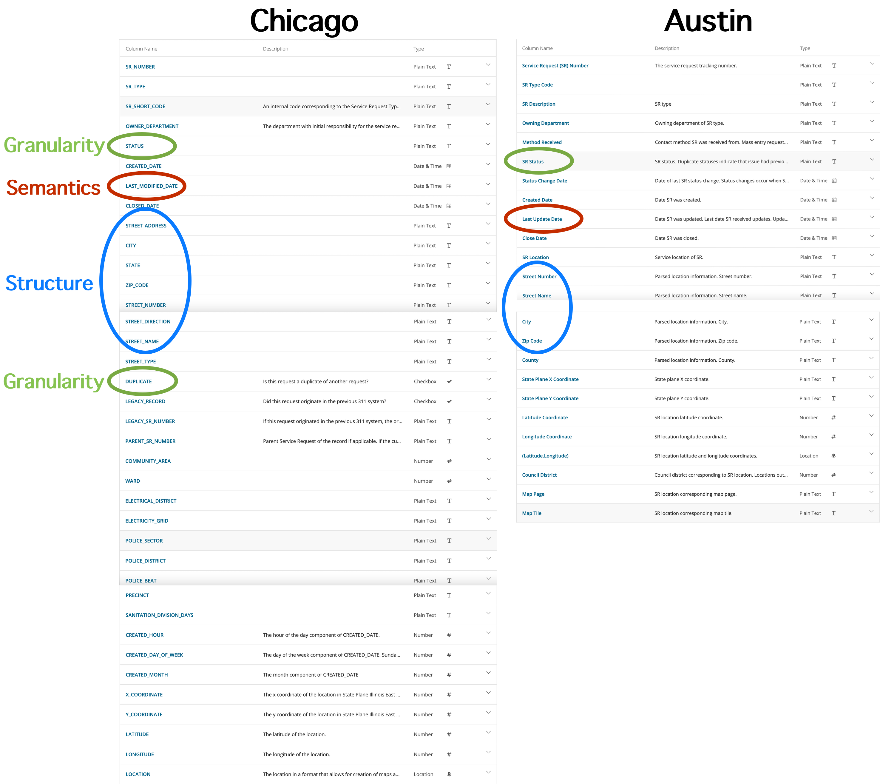
Even though these two cities record the same information about the same concept using the same data infrastructure (each city publishes data using a Socrata-based data repository) there are appreciable differences and challenges in integrating these two datasets. The annotations above point out some of these slight but appreciable differences:
Granularity
We can see that the Chicago dataset contains a variable Status. As of April 3, 2021, the column has no description, but if we perform a little magic with the API (more on this in a later module) we can see that the values in this field are:
[{"status":"Canceled"}
,{"status":"Completed"}
,{"status":"Open"}]
Additionally, there is a field called Duplicate with the following values:
[{"duplicate":false}
,{"duplicate":true}]
The Austin dataset contains a similar variable SR_Status with a description of “Duplicate statuses indicate that issue had previously been reported recently.” If we perform our API magic again, the values in the field are:
[{"sr_status_desc":"CancelledTesting"}
,{"sr_status_desc":"Closed"}
,{"sr_status_desc":"Closed -Incomplete"}
,{"sr_status_desc":"Closed -Incomplete Information"}
,{"sr_status_desc":"Duplicate (closed)"}
,{"sr_status_desc":"Duplicate (open)"}
,{"sr_status_desc":"Incomplete"}
,{"sr_status_desc":"New"}
,{"sr_status_desc":"Open"}
,{"sr_status_desc":"Resolved"}
,{"sr_status_desc":"TO BE DELETED"}
,{"sr_status_desc":"Transferred"}
,{"sr_status_desc":"Work In Progress"}]
So the Austin dataset uses one column to indicate status, including duplicate status, while the Chicago dataset uses two columns to indicate status, with the duplicate value being afforded its own column. Additionally, the Austin dataset is more granular in terms of the variety of statuses they record. To integrate these datasets we would need to decide both how to deal with the duplicate statuses AND we would need to determine which values were important to include and how we would crosswalk the differences. For example, would we collapse the “Closed - Incomplete”, “Closed - Incomplete Information”, “CancelledTesting”, “TO BE DELETED”, from the Austin dataset into the simpler “Closed” value used in the Chicago dataset? How would we determine if they had the same meaning?
Semantics
Both datasets include information about the most recent update (response) to the request, but these variables are labeled in slightly different ways - LAST_MODIFIED_DATE and Last Update Date. This seem like it should be fairly simple to tidy by renaming the data variable (but as we will see, this proves to be more more challenging than just renaming the variable).
Structure
Both datasets also include location information about the report. However, there is both different granularity as well as a different ordering of these variables. To tidy this location information, we would need to determine which variables to retain and which to discard.
The process of modeling our data tables before integration facilitates making accurate decisions, but also enables us to record those decisions and communicate them to end-users. A data dictionary, or a loose description of the contents of both tables, is often our first step in deciding which data cleaning activities we need to undertake for integrating data.
Determine the Observation Depth
In integrating two data tables there will likely be a difference in granularity of values. That is, even if the same variable is present in both datasets this does not necessarily mean that the same unit of measurement is used between the two data tables.
As curators, value granularity prompts a decision about what specificity is necessary to retain or discard in the new integrated table.
A simple example will make this clear. Imagine we have three tables Location A, Location B, and Location C. Each table contains the same variable BirthWeight, but the values for BirthWeight in each table have a different observational depth. In comparing the values for this variable we might even observe (presumably) different units of measurement.
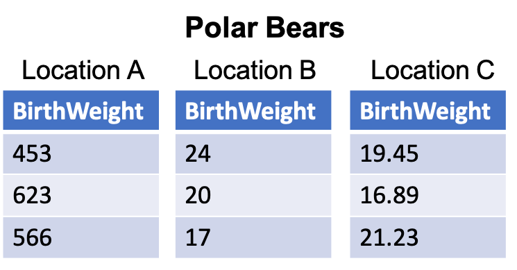
This example looks simple at face value, but will require an important decision for integration. Tables Location A and Location B both represent observational values of BirthWeight as integers but definitely of different units of measurement. Table Location C represents the observational values of BirthWeight as a decimal number most likely in the same unit of measurement as Location B.
Hopefully there is a data dictionary or text somewhere to indicate that the values in table Location A are in grams and the values in both tables Location B and Location C are in ounces. A best guess as to the different ounce values would be that table Location B values are rounded to the nearest whole number (ones place), while table Location C values are rounded to (or recorded as) the nearest hundredths place. Once we recognize these differences, our decision is two-fold. Should we convert the ounces to grams or vice versa and then will we use decimals or round to integers?
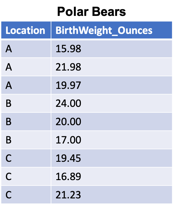
Regardless of our decision it is important to note that we are not just changing the values, but we are also changing their encoding - that is whether they represent integers or decimal numbers. (And we would need to document this change in our documentation). This may also affect their data type, for example Python has both integer and float (for decimal values) data types. Here is one possible integration solution:
Let’s look at differences in observational depth from two variables in the 311 data described above.
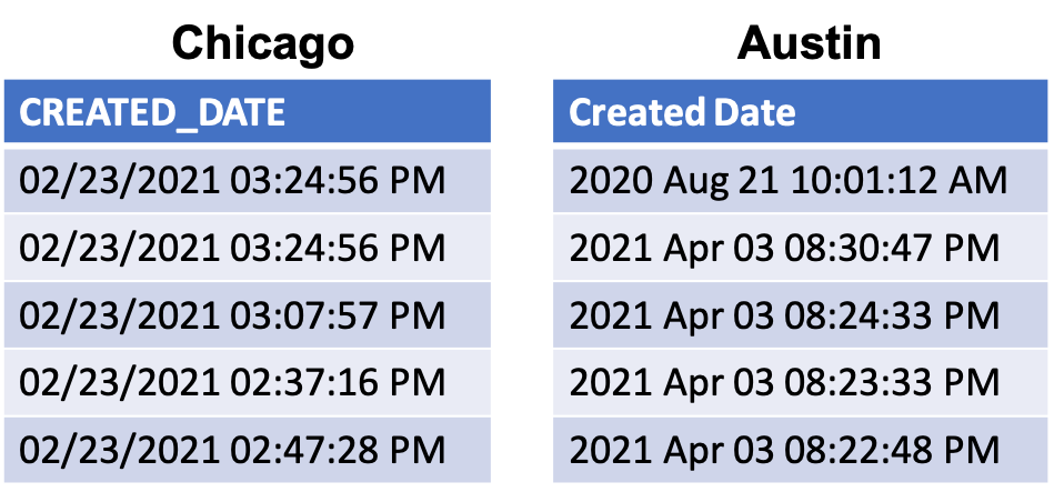
Chicago represents time of a 311 report following a MM/DD/YYYY HH:MM:SS 12HR form, while Austin represents this same information with YYYY MON DD HH:MM:SS 12HR
The observational depth (granularity) is the same in both tables but the formats of date in both datasets differ (and neither are ISO 8601).
If we want to integrate these two tables then we have to decide how to standardize the values.
Regardless of how we decide to standardize this data, what we have to try to retain is a reliable reporting of the date such that the two sets of observations are homogenous.
Determine Variable Homogeneity
The last integration precursor that we’ll discuss has to do with the homogeneity of a variable. In modeling two or more tables for potential integration we will seek to define and describe which variables are present, but we’ve not yet identified whether or not two variables can be reliably combined. To make this decision we need to first determine the goals of the integration. Some general criteria to consider when thinkng about the goals of integration are as follows:
- Analysis and Computation: If we are optimizing data integration for easing analysis then we want high amount of homogeneity in the variables we will combine.
- Synthesis: If we are optimizing for a more general purpose, such as the ability to synthesize results from two different datasets, then we can likely afford to combine variables that may have less homogeneity
- Statistical Significance: If we expect to create statistical summaries that require significant results (that is we will make some decision, forecast, or generalization based on our statistical analysis) then it is of the utmost importance that the combined variables have high homogeneity. But, if all that we require is a rough sense of when or where an observation occurs then low homogeneity is acceptable.
An example of variable homogeneity will help make these points clear. The Chicago and Austin tables each contain a variable that roughly corresponds with the “type” of 311 request or report being made. Both tables also contain a column with a short code. If we pay attention closely to the values in these two tables we can determine that the SR_Type and SR Description are homogeneous. That is, the Chicago table and the Austin table have similar information but use slightly different semantic values to control the variable.

Integrating these two variables in the same table seems possible, but we have a decision to make: We can either combine the two variables and leave the semantic value with low homogeneity, or we can create something like a controlled vocabulary for describing the type of 311 request being made and then normalize the data so that each value is transformed to be compliant with our vocabulary. For example, Traffic Signal Out Complaint in the Chicago table, and Traffic Signal - Maintenance in the Austin table both have to do with a report being made about traffic signals. We could create a broad category like Traffic Signals and then transform (that is, change the values) accordingly. But, we have only determined this step is possible by comparing the two variables directly.
When we determine there is a variable homogeneity that matches our intended integration goal we can then take a curation action. But, it is only through modeling, exploring observational depth, and investigating variable homogeneity that we can arrive at any one proper curation decision. It’s worth noting that the first two precursors - modeling and observational depth - don’t require us to necessarily have a goal in mind. We can start to engage in these activities before we quite know exactly what, or why we are going to integrate two tables. It is at the final step, variable homogeneity, that we start to formalize our goals and optimize our decisions as a result.
Horizontal and Vertical Table Integration
Thus far we’ve described precursors to making decisions and preparing data for integration. Once we’ve taken these steps we’re left with the practical task of combining the two tables. Generally, there are two types of table combinations that can be made: Horizontal and Vertical Integration.
Horizontal data integration
Horizontal data integration is necessary when we have the same set of observations, but multiple variables scattered across two tables. By performing a horizontal data integration we make a table wider by adding new variables for each observation. If you have any experience with databases this is also referred to as a join (for more information about SQL joins see this software carpentry lesson). To horizontally integrate data we perform left_joins or right_joins.
To accurately perform a horizontal data integration manually - that is copying and pasting between two datasets - it is necessary to make sure that each dataset has a shared variable. When we copy and paste one table into another, we can then simply align, or match, the two shared variables to complete the integration.
I am also going to show you how how to perform a horizontal data integration using R. You do not have to follow these steps unless you are interested. To follow along you should download and install the programming language R and the integrated development environment (IDE) RStudio (select the RStudio Desktop free installation). This example comes from friends running the Lost Stats project.
# Install dplyr - a package in the tidyverse for restructuring data
install.packages('dplyr')

# Load the library by calling it in your terminal.
library(dplyr)

# The data we will use contains information on GDP in local currency
GDP2018 <- data.frame(Country = c("UK", "USA", "France"),
                  Currency = c("Pound", "Dollar", "Euro"),
                  GDPTrillions = c(2.1, 20.58, 2.78))

#To view the data we have just created follow the next step
View(GDP2018)

# Now we will create a second data set that contains dollar exchange rates
DollarValue2018 <- data.frame(Currency = c("Euro", "Pound", "Yen", "Dollar"),
                              InDollars = c(1.104, 1.256, .00926, 1))
You will now have two tables that look something like this:
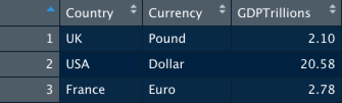
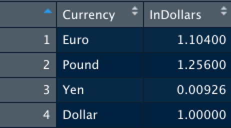
In the initial steps above we have created two data tables and assigned these tables to the name GDP2018 and DollarValue2018.
To horizontally integrate these two tables we want to join or combine GDP2018 and DollarValue2018.
Use help(join) to see the types of joins that we can make in R (and specifically look for the join help in the library dplyr).
To complete our horizontal data integration we simply do the following:
GDPandExchange <- left_join(GDP2018, DollarValue2018)

# We have now horizontally integrated our two datasets. To view this integrated dataset call the View function:
View(GDPandExchange)
The new table will look something like:
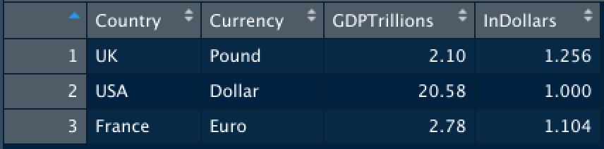
A helpful note appears thanks to dplyr that clarifies some of the magic that just happened:

The left_join (or any dplyr join) function will automatically detect that the Currency variable is shared in both data tables because it has the same column name. In recognizing this shared variable dplyr will use this, automatically, as the place to perform the left join. And helpfully, when dplyr detects this similarity, it simply retains just one example of the Currency variables and its values. Voilà - a single tidy data table through horizontal data integration!
Vertical data integration
Vertical data integration, which is much more common in curation, is when we have two tables with the same variables, but different observations. To perform a vertical integration we simply add new observations to one of our existing datasets. This makes our integrated data table longer because it contains more observations.
In R we first will subset a native data table (one that is included as an example) and then recombine it to see how vertical integration works in practice.
# Load the dplyr library so we can use its magic
library(dplyr)

# Load in mtcars data - a dataset that is native to R
data(mtcars)

# Take a look at the dataset and see what we will be first splitting and then recombining
View(mtcars)

# Split the dataset in two, so we can combine these back together
mtcars1 <- mtcars[1:10,]
mtcars2 <- mtcars[11:32,]

# Our machine is now holding the two tables in its memory - mtcars 1 and mtcars2.
# If you want to check this use the View function:

View(mtcars1)

# Use bind_rows to vertically combine the data tables
mtcarswhole <- bind_rows(mtcars1, mtcars2)

# The bind_rows command is simply concatenating or combing the two datsets one on top of the other.
# Now check to see the horizontally combined data tables
View(mtcarswhole)
These are the two most common integration tasks we will perform - integrating datasets with complimentary variables, and integrating datasets with new observations.
The hard part about data integration, as should be obvious by now, is in evaluating and preparing data to be combined. Once we have thoroughly completed each of the different integration precursors our task for actually integrating tables is relatively simple.
Summary
In this introduction to grand challenges in data curation we explored ways to prepare for and execute data integration at the table level. We first articulated a set of things that makes all data integration challenging:
- Differences in semantic content
- Differences in data structure and encoding
- Differences in data granularity
To overcome these challenges I proposed a set of integration precursors that included:
- Modeling data content
- Determining Observation Depth
- Determining Variable Homogeneity (it’s at this stage we start to formalize our integration goals)
Once these tasks were complete we looked at practical ways to combine two tables, including horizontal and vertical integration. We also were introduced to the magic of dplyr in performing simple data integrations in R.
Guest Lecture
This week we have a guest lecture by Kaitlin Throgmorton, MLIS who is a Data Curator and Bioinformatics Analyst at Sage Bionetworks. Kaitlin graduated last year (2020) and also took Data Curation I and II. Her lecture isn’t specifically about Data Integration but the concepts she introduces are important throughout the data curation cycle and I wanted you to have access to her talk sooner rather than later. It may seem hard to believe, but she was exactly where you are one year ago. I just wish this presentation could be in-person so you could ask her all your questions about the profession. But feel free to email her if you do have questions. I am extremely grateful that she was willing to put her time into this guest lecture.
Please open the video in a new browser window or tab to view. This slides for her talk are available openly in a Github repository.
Lecture
Instead of a traditional lecture this week, I’ve recorded a 15-minute presentation about a real-world data integration problem and solution from my own work. PDF of slides available.
Readings
Data integration is a topic that can be incredibly complex, and much of the published literature fails to make this an approachable or even realistic read for a course like DC II. But below are two readings that I highly recommend:
- This is a really detailed example of some serious curation activity. Don’t worry about understanding the nuances of the data, just read it for the example: Whong, Chris (2020) “Taming the MTA’s Unruly Turnstile Data”
- The Wikipedia article on data integration is a phenomenal overview that should compliment the content of this module
Optional
If you are interested in the history of this topic from the perspective of databases I also highly recommend the following:
- Halevy, A., Rajaraman, A., & Ordille, J. (2006, September). Data integration: The teenage years. In Proceedings of the 32nd international conference on Very large data bases (pp. 9-16). PDF
For a bit of historical background, Ch 1 of this book (pages 1-13) provides an excellent overview of how data were originally made compliant with web standards:
- Abiteboul, S., Buneman, P., & Suciu, D. (2000). Data on the Web: from relations to semistructured data and XML. Morgan Kaufmann. PDF
Exercise
The exercise this week was inspired by an interesting analysis of New York City 311 data by Chris Whong (archived tweet) last year at the beginning of the pandemic. What he observed was a 1000% increase in “Consumer Complaint” 311 requests since the first recorded case of Covid-19 infection in NYC. This was not without some important external conditions - after this recorded infection there was a more concerted effort by NYC residents to stockpile supplies. Having heard numerous informal complaints of price-gouging the city recommended that consumers report businesses using a 311 hotline.
A simple graph makes this more compelling than the narrative description - we see a huge spike in complaints beginning March 1st.

Inspired by this creative visualizing of 311 data and by the examples included in the content this week, you will be trying your hands at integrating 311 data from two different cities from a similar time period of March 1, 2020 through May 1, 2020. Lucky for us, there is an existing repository of 311 city data. However, retrieving data from some of these repositories can be difficult depending on the size of the data download and the ability to filter before downloading. So I am providing you with datasets to use. (If you’re really ambitious and have the time you are more than welcome to choose your own cities and download the data - but don’t prioritize this over other work for this class and other classes.) I have provided you with a random sample of 200 rows of data from San Francisco and 200 rows of data from Boston. (Note: you should be able to right-click on the pages that load from the links and Save Page As to open the content locally. But I will also upload the files to Canvas.)
Your exercise this week is to attempt to integrate (at least some) of the provided data. You may use your favorite tool for working with tables. Examples include: Microsoft Excel, Google Sheets, OpenRefine, R, Python. This task will be challenging but hopefully rewarding.
Here are some helpful pointers:
- Try to eliminate any unnecessary variables from your dataset. If we were trying to replicate Whoung’s analysis, for example, we really only need to retain the complaint description (and possibly a code or type similar to the
SR_SHORT_CODEfrom the Chicago dataset) and the date of the complaint. We don’t need all of the information about the data. - Try to find some similarities in the complaint descriptions across datasets. Are there descriptions you could combine / re-code?
- Consumer complaints may or may not exist in these datasets, so you don’t need to focus on that specifically.
- You do not need to perform data analysis or data visualization. The purpose of this exercise is to practice combine two datasets.
What to turn in:
Post the following in the discussion for this week’s exercise:
- Provide a table with an example of your integration. You do not need to integrate all 400 rows. Just choose an example to showcase the work you did. You can provide your new table via a Google Sheet, Excel document, .csv, or even a screenshot of the new table from whatever software platform you are using. If you were unable to integrate the the tables, show an example of the two tables and where you got stuck. I’m not promising that this will be easy, but I also don’t want you to spend hours on this. Take one hour to make your best attempt and then follow the next step.
- Provide an explanation (~1 paragraph) of what you tried to integrate the data, and why this was or was not challenging. Was this an example of vertical or horizontal integration (or a combination)?